Preface
Recently I've been learning how to perform JPEG encoding. I found many articles online, but discovered that very few explain every detail clearly, which led to many pitfalls during programming. So I plan to write an article covering the details with Python code as much as possible. For the specific program, you can refer to my open source project on Github.
Of course, this introduction and the code are not perfect, and may even contain some errors. It can only serve as an introductory guide, so please bear with me.
Various Markers in JPEG Files
Many articles have introduced the markers in JPEG files. I also uploaded a document with annotations on actual images (click to download) for reference.
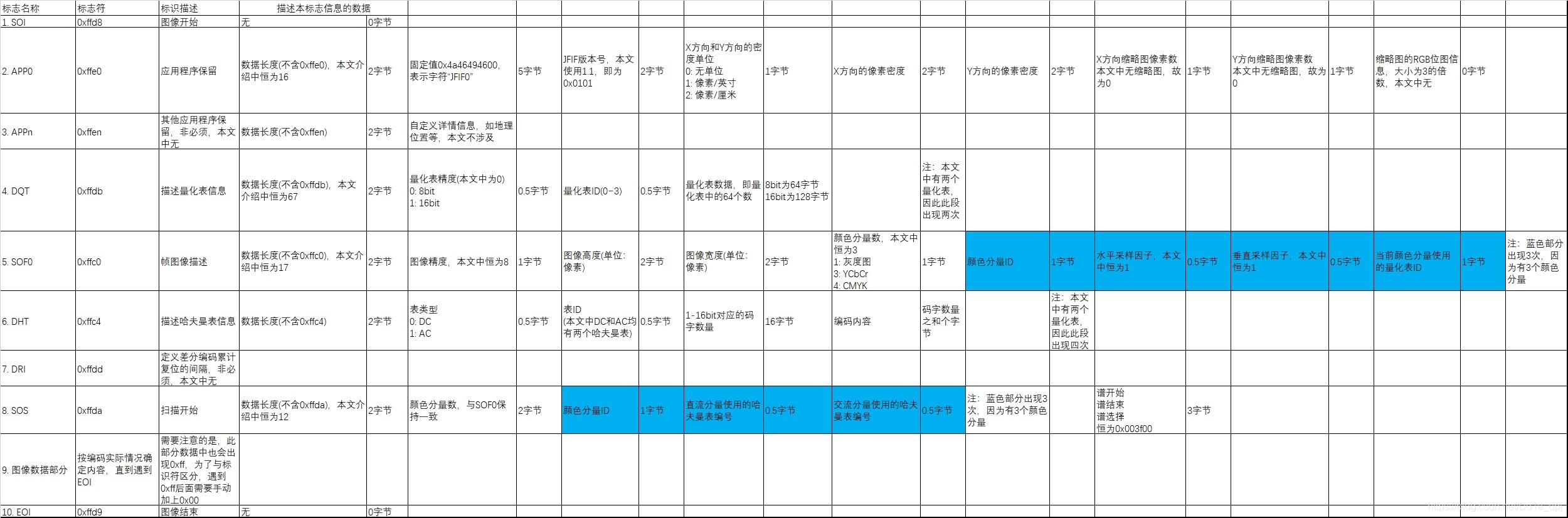
All markers start with 0xff (255 in hexadecimal), followed by bytes representing the data length of this block and data describing this block. See the figure below:
CodeBlock Loading...
At this point, we only have the image data left to write. But how exactly the image data is encoded, and how the quantization and Huffman encoding mentioned above are implemented, please see the next section.
JPEG Encoding Process
Since JPEG encoding requires 8*8 block processing of the image, this requires both the height and width of the image to be multiples of 8. Therefore, we can use image interpolation or sampling methods to make minor changes to the image so that both height and width become multiples of 8. For an image with thousands of pixels, this operation will not cause significant changes to the overall aspect ratio.
CodeBlock Loading...
Color Space Conversion
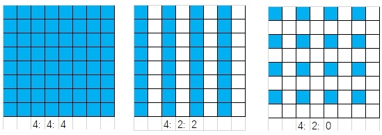
JPEG images uniformly use the YCbCr color space. This is because the human eye is more sensitive to brightness perception and less sensitive to chrominance perception. Therefore, we selectively increase the compression of Cb and Cr components, which can ensure the image appearance remains unchanged while reducing the image size to a greater extent. After converting to YCbCr space, we can sample the Cb and Cr color components to reduce their data points, achieving greater compression. Common sampling formats are 4:4:4, 4:2:2, 4:2:0. This corresponds to the horizontal and vertical sampling factors in the SOF0 marker. For simplicity, all sampling factors in this article are 1, meaning no sampling is performed, and one Y component corresponds to one Cb Cr component (4:4:4). 4:2:2 means two Y components correspond to one Cb Cr component, and 4:2:0 means four Y components correspond to one Cb Cr component. As shown in the figure below, each cell corresponds to one Y component, while the blue cells are the sampled pixel points for Cb Cr components.
The color space conversion formulas are:
All the above operations are rounded to integers. In 24-bit RGB bmp images, the R G B components all range from 0-255. Through simple mathematical relationships, we can easily find that Y Cb Cr components also range from 0-255. In JPEG images, we usually need to subtract 128 from each component so that the range includes both positive and negative values.
In Python, you can use functions from the opencv library for color space conversion:
CodeBlock Loading...
8*8 Block Division
In JPEG encoding, each 8*8 block is processed in order from top to bottom and left to right, and finally the data from each block is combined together. For the Y, Cb, and Cr color components of each block, the same operations are performed in the order of Y, Cb, Cr (using different quantization tables and Huffman tables).
CodeBlock Loading...
DCT Transform
DCT (Discrete Cosine Transform) converts spatial domain data to frequency domain for computation. This allows us to selectively reduce high-frequency component data in the frequency domain without significantly affecting the image appearance. Compared to Discrete Fourier Transform, Discrete Cosine Transform operates entirely in the real number domain, which is more advantageous for computer computation. The formula for Discrete Cosine Transform is:
Where . In JPEG,
Of course, you can also use functions from the opencv library:
CodeBlock Loading...
Quantization
After DCT transform, the DC component is the first element of the 88 block, low-frequency components are concentrated in the upper left corner, and high-frequency components are concentrated in the lower right corner. To selectively remove high-frequency components, we can perform quantization, which essentially divides each element in the 88 block by a fixed value. The elements in the upper left corner of the quantization table are smaller, while those in the lower right corner are larger. An example of a set of quantization tables is shown below (Y component and Cb Cr component use different quantization tables):
CodeBlock Loading...
Quantization process code:
CodeBlock Loading...
After quantization, many zeros appear in the lower right corner of the 8*8 block. To concentrate these zeros and reduce the data size through run-length encoding, we perform zigzag scanning next.
Zigzag Scanning
The so-called zigzag scanning essentially converts an 8*8 block into a 64-element list in the following order.
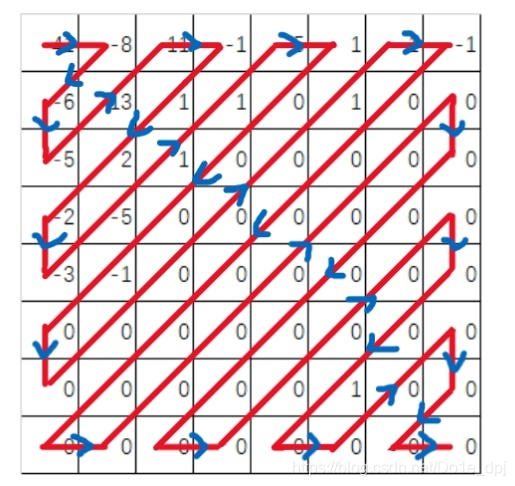
Finally, we get a list of length 64: (41, -8, -6, -5, 13, 11, -1, 1, 2, -2, -3, -5, 1, 1, -5, 1, 0, 0, 0, -1, 0, 0, 0, 0, 0, 0, 1, 1, -1, 0, 0, 0, 0, 0, 0, 0, 0, 0, 0, 0, 0, 0, 0, 0, 0, 0, 0, 0, 0, 0, 0, 0, 0, 0, 0, 0, 1, 0, 0, 0, 0, 0, 0, 0). All subsequent operations will use this list as an example.
Note that when storing the quantization table, we also need to perform zigzag scanning on the quantization table accordingly. Storing it in this format allows image viewers to decode the correct image (I spent a lot of time debugging this detail at the beginning). See the code for writing markers at the beginning of this article.
CodeBlock Loading...
Differential Encoding (DC Component)
The DC component values are often large, and the DC components of adjacent 8*8 blocks are usually very similar. Therefore, using differential encoding can save more space. Differential encoding stores the difference between the current block's DC component and the previous block's DC component, while the first block stores its own value. Note that differential encoding is performed separately for Y, Cb, and Cr components, meaning each component is subtracted from its corresponding previous value. We will introduce how to encode and store the DC component nowblockdc later.
CodeBlock Loading...
Run-Length Encoding of Zeros (AC Component)
After zigzag scanning, many zeros are grouped together. The AC component list is: (-8, -6, -5, 13, 11, -1, 1, 2, -2, -3, -5, 1, 1, -5, 1, 0, 0, 0, -1, 0, 0, 0, 0, 0, 0, 1, 1, -1, 0, 0, 0, 0, 0, 0, 0, 0, 0, 0, 0, 0, 0, 0, 0, 0, 0, 0, 0, 0, 0, 0, 0, 0, 0, 0, 0, 1, 0, 0, 0, 0, 0, 0, 0).
Run-length encoding of zeros stores two numbers each time. The second number is a non-zero number, and the first number is how many zeros precede this non-zero number. It ends with two zeros as the end marker (note especially that when the input data does not end with 0, two zeros are not needed as the end marker - this bug took me a long time to find, see line 23 of the code below). After run-length encoding, the above list becomes: (0, -8), (0, -6), (0, -5), (0, 13), (0, 11), (0, -1), (0, 1), (0, 2), (0, -2), (0, -3), (0, -5), (0, 1), (0, 1), (0, -5), (0, 1), (3, -1), (6, 1), (0, 1), (0, -1),(27, 1), (0, 0). This data length is 42, which is somewhat reduced compared to the original 63. Of course, the data chosen here is special. Actual data will have more zeros, or even all zeros, so the encoded size can be even smaller.
You may have noticed that (27, 1) is marked in red above. This is because in the encoding in Part 8, the first number is stored as a 4-bit number, so the range is 0-15. This obviously exceeds that, so we need to split it into (15, 0), (11, 1), where (15, 0) represents 16 zeros, and (11, 1) represents 11 zeros followed by a 1.
CodeBlock Loading...
JPEG Special Binary Encoding
After the above preparation, this section will introduce how the encoded DC and AC components are written to the file as a data stream.
In JPEG encoding, there is the following binary encoding format:
CodeBlock Loading...
For a number to be stored, we need to obtain the required bit length and the actual saved binary value according to the above format. Observing the pattern, it's not hard to find that the saved value of a positive number is its actual binary, and the bit length is also its actual bit length. The corresponding negative number has the same bit length, and the binary value is the bitwise NOT of the positive number. Zero does not need to be stored.
CodeBlock Loading...
For the DC component, assuming the value after differential encoding is -41, following the above operation, we can get its bit length as 6 and the saved binary data stream as 010110. For the value 6, we need to use canonical Huffman encoding to save its binary data stream. This part will be introduced in Part 9. Let's first assume the binary data stream for 6 is stored as 100, then the DC value for a certain color component of this 8*8 block is stored as 100010110.
After the DC component's binary data stream is written to the file, the AC values for this color component of the 8*8 block are encoded next. The values after run-length encoding are: (0, -8), (0, -6), (0, -5), (0, 13), (0, 11), (0, -1), (0, 1), (0, 2), (0, -2), (0, -3), (0, -5), (0, 1), (0, 1), (0, -5), (0, 1), (3, -1), (6, 1), (0, 1), (0, -1),(15, 0), (11, 1) , (0, 0).
First store (0, -8). For the second number, the same operation gives 4 bits and 0111. But unlike the DC component, we need to perform canonical Huffman encoding on 0x04, where the high four bits are the first number of (0, -8), and the low four bits are the bit length of the second number. Assuming 0x04 is stored as 1011 after canonical Huffman encoding, then (0, -8) is stored as 10110111. Next, perform the same operation for (0, -6) etc., and write the resulting data stream to the file in sequence.
Let's take another example (6, 1), where 1 is stored as 1, 1 bit. So we perform canonical Huffman encoding on 0x61, assuming it's 1111011, then (6, 1) is stored as 11110111. (15, 0) only stores the canonical Huffman encoded value of 0xf0.
After writing the data for one color component (assuming Y) following the above process, write the Cb color component data for this 88 block, then the Cr component data. Using the same method, after writing each 88 block data from left to right and top to bottom, write the EOI marker (0xffd9) as the image end.
Note: During the writing process, you need to check if 0xff is written. To prevent marker conflicts, we need to append 0x00 after it.
CodeBlock Loading...
Canonical Huffman Encoding
In this article, there are 4 canonical Huffman encoding tables, used for luminance DC component, chrominance DC component, luminance AC component, and chrominance AC component respectively.
CodeBlock Loading...
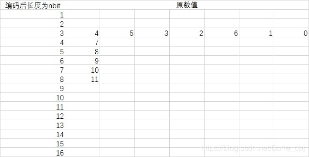
As shown in the code above, stdhuffmanDC0 etc. are the actual values saved in the markers. See the code in the marker introduction section for details. The first 16 numbers in this sequence (0, 0, 7, 1, 1, 1, 1, 1, 0, 0, 0, 0, 0, 0, 0, 0) represent how many numbers have encoded lengths of 1-16 bits, and the following 12 numbers are exactly the sum of the first 16 numbers. stdhuffmanDC0 actually describes the following figure:
Now we only know the data length after encoding each original data, but not what it actually is.
Canonical Huffman encoding has its own set of rules:
- The first code of the minimum encoding length is 0;
- Codes of the same encoding length are consecutive;
- The first code of the next encoding length (assuming j) depends on the last code of the previous encoding length (assuming i), that is
a=(b+1)<<(j-i).
From rule 1, we know that the code for 4 is 000. From rule 2, the code for 5 is 001, the code for 3 is 010, the code for 2 is 011..., and the code for 0 is 110. From rule 3, the code for 7 is 1110, the code for 8 is 11110...
CodeBlock Loading...
The final Huffman dictionary is quite long. You can view it in my github project. Finding the pattern will help you understand why the dictionary index in the write_num function is calculated that way.